Previous chapter Next Chapter

Key Symbols
Indexes and Other Signs
Abbreviations

2.2.1 Axisymmetric Flow in the Axial Turbine Stage

Assume that in the flow path of the turbine:

• The flow is steady relatively to the impeller, rotating at a constant angular velocity ω about the z-axis or stationary guide vanes.
• The fluid is compressible, non-viscous and not thermally conductive, and the effect of viscous forces is taken into account in the form of heat recovery in the energy and the process equations, i.e., friction losses are accounted energetically.
• If the working fluid is real (wet steam) it is considered the equilibrium process of expansion.
• the flow is axisymmetric, i.e., its parameters are independent of the circumferential coordinate.

Under these assumptions the system of equations describing the steady axisymmetric compressible flow motion, includes:

1. The equation of motion in the relative coordinate system in the Crocco form

2. Continuity equation

3. The equation of the process or system of equations describing the process

4. The equations of state

5. The equation of the flow surface

where n ⃗’ – normal to the S₂ surface (Fig. 2.1).

6. The equation of blade force orthogonality to the flow surface

Projections of the vortex in the relative motion rot W ⃗’ = ∇ * W ⃗’ to be determined by the formulas:

Taking into account (2.12), projection of the equation of motion (2.6) on the axes of cylindrical coordinate system can be written as follows:

• On the r axis (radial equilibrium equation)

• on the u axis:

• instead of the projection on the z axis will use energy conservation equation:

The components of the relative velocity based on the designated flow angles (Fig. 2.1) can be written as

From the relation  [ n ⃗’ , F ⃗’ , ] = 0 will have:

We express the ratio of the normals projections through the flow angles (Fig. 2.2):

Than we can write

Transforming the radial equilibrium equation

transformed into

The last expression, in turn, by shifting from the coordinates s, n to coordinates s, r is represented as:

since

 

The projection of the equation of motion in the circumferential direction

Let us now consider the projection of the equation of motion (2.6) in the circumferential direction (2.14). Using (2.16), and the relationship between the coordinates z, r and s, r in the meridian plane

equation (2.14) becomes:

• for a given c_ur (inverse problem):

• in the gap between vanes (free channel):

• for a given β

These equations enable us to determine the projection of the blade force F_u in the circumferential direction. The radial component F_r is expressed through the circumferential according to (2.17).

The projections of the friction force on the coordinate axes

The expression for the friction force

can be transformed by using the expression (2.16) and the binding ratio between the cylindrical coordinates z, r and the coordinates s, r:

whence we get the projection of the friction force on the coordinate axes:

The continuity equation is advisable to use in a form

For a free channel from the projection of the equation of motion in the absolute coordinate system to the circumferential direction, obtain, that the circulation c_ur = const along the meridian streamline and

Then for a free channel (χ = 1) from (2.31) we have:

2.2.2 Aerodynamic Calculation of the Axial Turbine Stage in Gaps

The considered above in the general formulation, the problem of calculation of axisymmetric flows of a compressible fluid in the flow path of the axial turbine can be simplified and reduced to the calculation in gaps [9]. The flow in the axial gap is seen at the main proposals set out above. Within axial gap in the space free of the blades (χ = 1); because of its small length in the axial direction the entropy S locally do not changes along the meridian streamlines

it is possible to force components F_r= f_r = 0;stream keeps the direction of motion, telling him by blades (i.e., the angle of the flow β is et).

In these assumptions the radial equilibrium equation will differ from (2.24) in the absence of the right side of F_r= f_r:

 

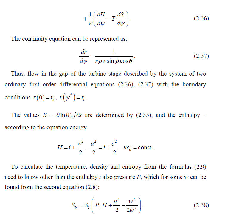
Consequently, the system of equations, describing the steam flow in the axial turbine stage gaps are as follows:

• after the guide vanes:

The numerical realization of the stage thermal calculation problem

Mathematical models of axial turbine stages, discussed above, allow their calculation by setting some additional (closing) relations, for example, the
distribution of the angles β and α (direct problem), the quantities c_ur, pc_z et al. (inverse problems).

To solve the direct problem of stage calculation in gaps the following information is required:

• • form of the stage meridian contours, i.e. external and internal radii of axial
    sections;
  • rotor speed ω;
  • stagnation parameters at the stage input P^*₀ and i*0
  • the geometrical characteristics of the blades: entry and exit angles, as well as blades count in the crowns, the chord, edge thickness and other parameters necessary for determining the velocity coefficients along the blade length;
  • if the velocity coefficients are predefined – their distribution along the
    blade length.
  • streamline slope angles θ and their curvature ℵ in fixed axial sections.

There are varieties of the direct problem with a given flow rate G and with a specified back pressure P₂ Solution of the problem with a fixed flow easier because the integration of the equations (2.39), (2.40) is made for a known ψ^*=G/(2π) value and mathematically formulated as a two-point boundary value problem for a system of two ordinary first order differential equations of the form:

The solution of (2.43) is made in two stages: first, the first equation is solved and the distribution of the flow in fixed axial gap is found, then, knowing the parameters entering the impeller can solve the second equation. That is, the problem is reduced to determining the roots of the equation with one unknown for each of the two equations (2.43). For the calculation of the subsonic solutions of (2.43) can be successfully used the methods of nonlinear programming. The system (2.43) is solved by sequential minimization of residuals

using one of the described one-dimensional extremum search methods.

Solution of the problem with a given back pressure  P₂ (flow rate unknown) is more complicated. To determine the unknown mass flow G to the system of equations (2.43) is necessary to add one more thing – a limit on the heat drop.

In this formulation of the problem it seems appropriate to set the mass flow averaged pressure according to the formula

In view of (2.45) to calculate the level with a given back pressure is needed to solve a system of three equations with three unknowns:

Numerically, the problem is solved to minimize the sum of squared residuals

A maked up mathematical model describing the flow in the axial gaps of turbomachine (equation (2.39), (2.40)), allows the calculation of supersonic flow (including the transition through the speed of sound), which M_s <1, i.e.,in the case of the meridional component of velocity less than the velocity of sound. Specified the conditions satisfy all existing stages of powerful steam turbines.

Calculation of supersonic stages must be performed with a given back pressure, because otherwise does not provide a unique solution of the equation of the form (2.41). At the same time, the system of transcendental equations (2.46) in the variables c_1h,w_2h,ψ^*.in contrast to (2.43) has a unique root.

Another feature of the supersonic stages calculation is the need to consider the flow deflection in an oblique cut at Mach numbers higher than unity. For this purpose it is possible to use a method of determining the flow deflection angle in an oblique cut comprising in equating flow rate into the throat section and behind the blade [10, 11].

In this case, to calculate the residuals of equations (2.44), (2.46) it is necessary to integrate the system of ordinary differential equations of the form (2.41), namely (2.39), (2.40). These equations are due to the complexity of the form of the right sides in the general case can be integrated numerically. When integrating (2.39) (2.40) should be borne in mind that at each step of pressure shall be determined by solving the equations of the form (2.38), which greatly complicates the task.

Finally, we note that because of the existence of the right sides of (2.38), (2.40), a member

,  the system, generally speaking, can not be considered as written in the form of Cauchy, as these non-linear supplements are some of the functions w₂ or c₁, r and their derivatives. When integrating these terms are determined by successive approximations.

The important point is the choice of numerical methods for integrating systems of the form (2.41). Extensive experience in solving such problems suggests the possibility of partitioning the integration interval to a small number of steps (5–10). As a result of numerical experiments comparing different methods, preference was given to the modified Euler’s method [12], which has
the second order of accuracy for the integration step.

The leakage calculation is necessary to conduct together with a stage spatial calculation, the results of which are determined the parameters along a height in the calculation sections, including the meridian boundaries of the flow part.

The stage capacity depends on the value of clearance (or leakages), in connection with which calculation of the main stream flow is made by mass flow amplification at fixed the initial parameters and counter-pressure on the mean radius, or with counter-pressure elaboration at fixed initial parameters and mass flow.

The need for multiple steps in optimization problems requires a less labor-capacious, but well reflecting the true picture of the flow, methods of axisymmetric stage calculation. Its main point is to calculate the stage parameters in the axial gaps supplemented by the algorithm of stream lines slope and curvature refinement in the design sections.

When calculating the stage taking into account leakage, the continuity equation is convenient to take the form:

where μ– mass transfer coefficient, which allows to take into account changes in the amount of fluid passing through the crowns, and at the same time to solve a system of ordinary differential equations

As shown, the calculation of spatial flow in the stage with the known in some approximation the shape of the stream lines is reduced to the solution in the sections

(Fig. 2.3) of a system of ordinary differential equations (2.39) and (2.40), where as independent variable a stream function ψ is taken. Thus, the equations describing the flow in the axial gap, presented in the form of:

• in the section after the guide vanes:

• in the section after rotor:

The solution of the boundary problems (2.49), (2.50) for a given mass flow rate is reduced to finding the roots of the two independent transcendental equations (2.43) with respect to the hub velocities c_1h,w_2h.

For a given backpressure to the number of defined values the mass flow ψ^* is added and the problem reduces to solving a system of three equations. As a third equation the stage heat drop constraint is added (2.45) that can be symbolically written as

Systems of equations are solved using the methods of nonlinear programming.

An approximate method of meridian stream lines form amplification using their coordinates in the three sections, is to construct an interpolation cubic spline at a given slopes at the flow path boundaries. In order to accelerate the convergence the stream line curvature is specified with lower relaxation. Previous calculations showed that the interpolation process converges with sufficient accuracy in 3…5 iterations.

Mass flow rates through crowns carried out in parallel with the streamlines construction. The algorithm allows to solve the direct problem of the spatial stage calculation in the gaps in various statements, with given or variable in the process of calculating the streamlines, velocity and flow coefficients of crowns, at various ways of flow angles distribution along the height, for a perfect gas or steam.

The algorithm was tested by comparing the calculation results with the exact solutions, as well as with the experimental data obtained for a large number of stages of the experimental air turbines in the turbine department of NTU “KhPI” [13–14, 15]. The results of calculations and experiments illustrated in Fig. 2.4–2.12. It should be stated a good calculations agreement with the experimental result for the various stages of the different elongation, meridian shape contours, twist laws and the reaction degree at the mean radius.

The greatest difficulty to calculate present stages with the steep opening of the flow path (Fig. 2.12), and the cylindrical stages with inversely twisted guide vanes (Fig. 2.4, 2.6–2.8).

The calculation of stages with inverse twist using the proposed method allows to obtain a valid gradient of reaction degree and circumferential velocity component of the stage, while the calculation provided in assumption of cylindrical flow gives results that differ significantly from the experimental data (Fig. 2.6–2.8). The technique allows to take into account also the effect of the
law of the impeller’s twist on the distribution of parameters in the gap between guide vane and rotor. This is evidenced by the comparison stages 41 and 42 (Fig. 2.7, 2.8) with the same nozzle unit, the first of which has a cylindrical impeller, and the second – twisted by constant circulation law.

2.2.3 Off-Design Calculation of Multi-Stage Steam Turbine Flow Path

Formulation of the problem

The off-design analysis problem is to determine the gas-dynamic characteristics derived from the design calculation such as the size of the flow path (FP) and the parameters that determine the long-term (steady) operation of the turbine. The need to analyze FP off-design modes arises when assessing aero- and thermodynamic, power, strength parameters of the turbine in extreme operating conditions, the choice of method for control and calculation of steam distribution, for turbines designed to operate at changing the regime parameters (speed, unregulated steam extraction and so on).

The specifics of these problems requires a gas-dynamic calculations in a direct statement, which is more labor intensive than the calculations commonly used in the design stage. In connection with this methods designed for use with a computer optimization procedures must meet several requirements:

• to base on the equations of motion of a real working fluid in the flow path
  of the multi-stage turbine;
•  to consider with the required accuracy the influence of geometrical and
  operational parameters on the loss factors of the FP elements;
• to allow to conduct calculations with varying from section to section the
  mass flow rates;
• to be highly reliable and economical in terms of consumption of computer
  resources, i.e. make it possible to carry out multi-variant and optimization
  calculations.

To calculate high, medium and, to a lesser extent, the low-pressure parts of powerful steam turbines, justified the use of one-dimensional gas dynamics calculations using the simplified radial equilibrium equations in a axial clearance, the leaks balance at the root of the diaphragm design stages and the calculation method of the FP moisture separation. Accounting for the loss of
kinetic energy and efficiency assessment should be carried out by successive approximations based on the current results of the gas-dynamic calculation and empirical relationships, and reliability of the results – achieved by comparison with experimental results and the introduction of necessary adjustments.

Should be regarded as a satisfactory the accuracy of coincidence of calculated and experimental values of the relative losses in the range of 5…7% for FP made with straight or twisted by constant circulation law blading in the absence of the sharp curvature of the meridian contours. When the actual loss levels of 10…30% error in determining the efficiency, thus lies in the range of 0.5…2% [15].

Method of calculation

One-dimensional steady-state equilibrium adiabatic motion of water vapor in the flow path in a coordinate system rotating with angular velocity ω, sought a system of equations:

 

The solution to this system of equations for an isolated axial turbine stage in a direct statement requires:

The two main statements involve mass flow G₀ determination at certain stagnated pressure P^*₀ at stage inlet, or the P^*₀ definition at known flow rate. It is also possible the solution of the problem with given at the same time G₀ and P^*₀ changing angles α_1e or  β_2e in particular, makes it possible to simulate the nozzle assembly with rotary blades. In all cases, subject to the definition of the flow speed c₁ and w₂.

For definiteness we shall consider the problem with fixed P^*₀ and mass flow determination. We transform the equation of continuity (2.52) for the nozzle in view of (2.51), (2.53), (2.54):

Under α₁ and β₂ at subsonic flow understood the cascade’s effective angles, and at supersonic – flow angles in the oblique cut-off by the Ber formula.

The third equation is:

Under certain velocity factors φ and ψ to determine the unknown c₁ , G, w_1,  there are three equations (2.55)–(2.57), which in general terms be written as follows:

The system (2.58) is solved numerically by minimizing the sum of squared residuals g₁ ² +g₂ ² + h ² using the conjugate gradient method.

Calculation of multistage flow path does not differ systematically from the stage calculation. An equation of (2.58) is written for each of the stages, which leads to a system of the form

where j – stage index; n – number of stages in the FP.

The numerical solution is carried out by minimizing the function

by 2n + 1 unknowns  c_1j,w_2j, (j = 1, …,n) + h²

Sections may have different mass flows because of the leaks, district heating or regenerative steam extraction, moisture separation and so on. In the equations (2.59) in this case instead of a mass flow rate G in the relevant sections should take the current value

where ΔG_k– given or confirmed in iterations the mass flow change in the transition from (k – 1) section to the k-th (k=1…2n).

The unknown is considered the G₀ mass flow at the FP entrance.

After the solution of (2.58) or (2.59) all the parameters of the flow calculated, loss factors and the actual mass flows in sections adjusted. The required number of iterations is usually equal to 3…4.

Kinetic energy loss determination

Losses associated with the leakage of the working fluid are considered separately. The remaining components are divided into losses in cascade and auxiliary, which are allocable to the stage heat drop.

Methods of assessing the losses in cascades based on research [8, 16] with a corresponding adjustment of empirical dependencies using test data about profiles used in the turbine building [17, 18].

Corrections for the Reynolds number, angle of attack, the thickness of the trailing edge, at supersonic flow are taken over without change [19]. The amendment to the angle of attack in the profiles provided with an extension of the leading edge, is estimated according to experimental studies on the standard nozzle profiles and the impact of the extension on the profile loss – NPO CKTI the procedure [20].

The basic component of the profile X_pb obtained by a corresponding adjustment to the loss level of graphic dependence [16]. Basic secondary loss is determined by the corrected chart [16], an amendment to the ratio of the chord to the height of the blade N_b/l  – according to [16], and the coefficient N_s taking into account the length of the visor hanging over the trailing edge of the blade – based on experimental data on nozzle standard profiles test data.

When assessing the energy losses in the rotor blades, can be taken into account the effect of the periodic incident flow unsteadiness caused by the presence of traces of the previous nozzle cascade, as amended N_y. The degree of non-uniformity of the incoming flow is taken over [8].

Additional energy losses are the disc friction and ventilation, extortion, humidity, the presence of the wire bonding and friction in the open and closed axial clearance in accordance with the guidelines [21].

Leak sand leakage losses calculation

It is estimated that losses caused by leakage of the working fluid into the gaps of the flow path, associated with a decrease in the mass flow rate through the crowns, aerodynamic and thermodynamic mixing with the main flow losses, as well as the deviation of the kinematic parameters in the gaps comparing to the design.

To determine the thermodynamic parameters near the flow path margins, needed to calculate the leaks mass flows, a simplified equation of radial equilibrium

is involved. In the gap between vanes considered that c_ur = const, P₁ = const , and behind the stage c2_u = const, P₂ = const.

Leaks in the root area of multistage flow paths are the solution of the mass flow balance equations through diaphragm, root seals and discharge holes taking into account given dependences of the gaps flow factors and friction coefficients of the regime and geometrical parameters, changes in pressure and flow swirling in the disk chambers along the radius at the presence of the working fluid flow etc.

Evaluation of leakages based on a calculation of the anterior chamber only, first, does not allow correct balance the mass flows along the FP, and secondly, may lead to considerable errors as the leakage values and axial forces, particularly at the off-design operation.

The algorithm is developed for the calculation of leakages in multistage FP, in which can be built leaks circuit within the cylinder based on the majority of the factors, influencing them [14]. Calculation of mixing the main flow with leaks through tip and root gaps is based on the balance equations for flow, enthalpy, and entropy. Raising the equations of motion for the evaluation of aerodynamic mixing losses allows, under certain assumptions, take into account the impact on the mixing loss of the blowing working fluid angle.

The third group of losses factors, caused by leaks, mainly, through a change of velocity coefficient of cascades after gaps, where mixing occurs, due to variations of inlet flow angles.

2.2.4 Simulation of Axisymmetric Flow in a Multi-Stage Axial Turbine

To solve this problem, we used a combined one-dimensional and axisymmetric approach.

A mathematical model of a coaxial flow of the working fluid in the flow part of a multi-stage axial turbine

This model belongs to the class of quasi- two-dimensional models, and is a logical continuation of the one-dimensional model of the FP shown in subsection (2.2.3). All equations, methods and techniques of assessment of energy dissipation in the elements of FP used in the one-dimensional model, have been fully utilized in the development of quasi- two-dimensional model of the coaxial FP.

A distinctive feature of the coaxial model is the fact that the system of equations (2.59) are determined not to cross-sections corresponding to the mean radius of the multistage FP crowns, and for each current streams along its midline.

The system of equations (2.59) in a coaxial FP model in a general form as follows:

where m – is equal to increased by two the number given sections (streamlines) along the radius of the blades; j – number of cross-section along the blade height (the first cross section is located at the root level).

Accordingly, the dimension of the system of equations in a mathematical model of a coaxial flow in the FP is equal to (n + 1)m.

The marked increase in the number of sections required for a significant approaching of the root and near-the-tip stream lines to the root level and the peripheral area, respectively. With the same purpose the cross sectional area of the extreme stream lines assigned minimum values (1% of area of the corresponding vane). For the first iteration the remaining cross-sectional areas between the stream lines are equal and are determined as follows:

S_(k,j)=0.98S_(k)(M-2),

Where S_(k)  – cross-section area of k-th vane.

After determining the S_(k,j) are determined the radii of mean lines of all flow streams, angular velocities and the values of all the geometric characteristics of the cascades at those radii. In subsequent iterations, the average radius of the stream lines, and all the characteristics of cascades and the working flow determined in accordance with the obtained distribution of the mass flow the radius of corresponding vanes. This ensures the equality of the working fluid (including the extractions and leakages) along the respective stream lines.

Considering that the system of equations (2.62) is based on the onedimensional flow theory for each stream line, where there is no equation of radial equilibrium, it becomes apparent that the above-described method of stream tubes sizing, is most accurate by using this model, it will be possible to evaluate the characteristics of the axial turbines, which vane’s twist corresponds
to the S_ur = const law, or close to it. For practical tasks coaxial mathematical model is most suitable when assessing the characteristics of the high pressure cylinder (HPC) flow path.

Despite the fact that the flow of working fluid along each stream tube in consideration of coaxial mathematical model of the FP is modeled in accordance with the one-dimensional theory, when calculating the flow kinematics the slope angles of each stream line are taken into account (curvature of the streamlines is not considered) and identifies all components of the flow velocity in axial gaps. To determine the angles of the middle line of the stream tubes cubic spline interpolation is used. A well-known feature of these splines is the coincidence of the first and second derivatives of the neighboring areas in the nodes of the spline coupling. It allows us to describe the midline of a stream line using dependence, which provides its most smooth shape.

Because in the outer iteration loop of the multistage axial turbine FP coaxial mathematical model (as well as in the one-dimensional mathematical model of the FP), the quantities of moisture separation, tip leakage and near-the-hub leakages and the working fluid extractions to the heating system and feed-water heating refer to the entire stage, and not to each stream tube, the question of adequate distribution of the marked mass flow changes between the stream tubes arise.

In this case, there are two variants of distribution of leaks and the working fluid extractions between the stream tubes:

1. The total change in the mass flow of the working fluid in the transition from one vane to another distributed between streams in proportion to their cross-section areas (1-st iteration).
2. The distribution of mass flow changes in proportion to the stream tube mass flow, the size of which is determined from the condition that the mass flow of each stream tube in accordance with the law of the flow rate changing along the radius of the stage, obtained in the previous iteration.

Additionally, there are also two versions of the distribution of secondary loss of height of the blade:

1. The secondary losses are concentrated at the ends of the blades.
2. The secondary losses are evenly distributed among all streams tubes (proportional to the mass stream tube mass flow).

Integral indicators of each stage in the coaxial model are determined by the relationships below:

A mathematical model of an axisymmetric flow of the real working fluid in a multi-stage axial turbine FP

Despite the fact that the coaxial mathematical model of the flow of the working fluid in the FP, as described in the previous section, has a fairly narrow range of independent use, yet it has a sufficiently high potential. If the formation of the transverse dimensions of the stream tubes to carry the light of the decision of the radial equilibrium equation (sections 2.2.1, 2.2.2), this model can be successfully used in the calculation of axisymmetric flow in a multistage axial turbine FP with virtually any kind of its crowns twists.

The use of coaxial FP model to evaluate the distribution of the static pressure behind the rotor blades to determine disposable heat drops of each stage that you need to solve the axisymmetric problem “with a given back pressure”. It is known that only in such a setting is possible to find the correct solution to supersonic stages. Marked problems for each crown of multi-stage flow path solved by the means of stream line curvature method. Thus, in view of (2.46) and the system of equations (2.62), the scheme for solving the problem “with a specified back pressure” for a multi-stage axial flow turbine parts will be as follows:

• Using a coaxial FP model made an initial assessment of the static pressure distribution along the radius of the stages working crowns.
• Relations obtained according to the static pressure of the stages as the boundary conditions are transferred to the axisymmetric simulation unit
  (sections 2.2.1, 2.2.2).
• As a result of solution of the boundary value problems (2.49) and (2.50), for each stage the distributions of the mass flow of the working fluid along the nozzle and working crowns radii for all FP stages are formed.
• The resulting distributions of the mass flow of the working fluid along the radii of the crowns are used to determine the average of the radii of new stream tubes and areas of cross-sections for the coaxial FP model.
• Calculation of coaxial FP model with the new values of the transverse dimensions of the stream tubes is performed.

For clarity, the above-described sequence of solving axisymmetric problem “with a given back pressure” for multi-stage FP is shown in Fig. 2.13.

Consider some features of the numerical solution of axisymmetric problem for multi-stage FP. First, in dealing with this problem it is necessary to determine the parameters of the working fluid along the streamlines for multistage FP with variable from crown to crown mass flow of the working fluid. The marked change often occurs in the steam turbines FP, where the extraction of the working fluid is carried out between the stages, for example, for the feed water heating or a heat supply needs.

As the result of boundary problems solutions (2.49) and (2.50), the mean radii of stream tubes for all the crowns of multistage FP are transmitted to the coaxial model, where for the new stream tube’s cross-sectional areas, angular velocities, and all the geometric characteristics of the nozzle and working blades, the FP calculation is carried out and the new static pressure distribution after
working stages crowns is determined.

The FP calculation results using the algorithm corresponding to the coaxial model again transferred to the block of boundary problems solutions (2.49) and (2.50). Described iterative process continues as long as the results of the calculation for both FP calculation algorithms differ less than a prescribed accuracy. Thus, the FP coaxial model and boundary value problems (2.49) and (2.50) complement each other in solving the axisymmetric problem, eliminating the “alignment” on the results of the one-dimensional calculation and more adequately assess the value of disposable heat drop of FP stages.

It should be noted that the numerical implementation of the axisymmetric mathematical model of the working fluid flow in the FP in the form of alternate use of coaxial mathematical model and boundary problems, can with a high degree of adequacy and accuracy to model the processes in the FP with stages with relatively long blades and having a twisted crowns substantially different
from the law c_ur = const.  As an example, in Fig. 2.14 are shown the shape of the flow lines resulting from the calculation of LPC FP of powerful steam turbine using the above axisymmetric mathematical model.

2.2.5 Cascades Flow Calculation

For the design of high efficiency axial flow turbines flow path it is important to have accurate, reliable and fast method for calculation of cascade flow and friction loss on the profile surfaces.

In the calculation of subsonic flows of an ideal liquid in the cascades long used an approach based on the reduction of partial differential equations to Fredholm integral equation of the 1-st or 2-nd kind [8, 22]. Available numerical implementation of solutions to these equations are facing a number of problems that do not allow a sufficient degree of reliability or accuracy of the calculated
arbitrary configuration cascades.

For example, for a long time, we used the method of calculation [22] reduces to the solution of the integral equation of the second kind with respect to the speed potential. It is possible to solve a number of important practical problems of cascade optimization, but had important shortcomings: the complexity of the integral equation kernel normalization, which led to difficulties in calculating thin and strongly curved profiles, as well as the need for numerical differentiation calculated potentials, which brings an additional error in the profile velocity distribution.

Later, we developed a method for cascades potential flow numerical calculating with an approximate view of the ideal gas compressibility based on the solution of the Fredholm equation of the 2-nd kind with respect to speed on the rigid surface, and a program for the PC is designed to work interactively.

Friction loss on the profile is carried out by calculating the compressible laminar, transitional and turbulent boundary layers using one-parameter Loitsiansky method [23]. To improve the accuracy of the results obtained on the basis of the recommendations given in the literature, calculated buckling points and end of the transition from laminar to turbulent boundary layer depending on the pressure gradient, the degree of free-stream turbulence and of profile surface roughness.

The developed algorithms for an ideal fluid flow calculation in the cascade and the boundary layer on the surface of the profile give a good qualitative and quantitative agreement between the calculated and experimental data for different types of cascades at different inlet angles, relative pitch, Mach and Reynolds numbers, characterized by high speed and are therefore suitable for
use in problems of optimizing the axial turbomachinery blades shape.

2.2.6 Computational Fluid Dynamics Methods

Aerodynamic optimization of turbine cascades is directed search a large number (hundreds to thousands) variants for their geometry, which increases with the number of variable parameters. The most reliable source of objective data on the flow of gas in a turbine cascade – physical experiment – obviously can not provide a sufficiently deep extreme.

Therefore, currently in the works for aerodynamic optimization it is the most popular approach in which to obtain data on the nature and parameters of the flow of the working fluid in the tested inter-blade channels numerically solve the Navier-Stokes equations, or their modifications [24].

Navier-Stokes equations written in conservative form is as follows:

Since the analytical solution of this system of equations associated with insurmountable mathematical difficulties, such a direction as computational fluid dynamics (CFD) arose, which deals with the numerical solution of the Navier-Stokes equations. The numerical solution of the equations of fluid dynamics involves replacing the differential equations of discrete analogs. The main criteria for the quality of the sampling scheme are: stability, convergence, lack of nonphysical oscillations. Computational fluid dynamics is a separate discipline, distinct from theoretical and experimental fluid dynamics and complement them. It has its own methods, its own sphere of applications, and its own difficulties.

Given the speed of modern computers, the most appropriate approach is based on a system of Reynolds-averaged Navier-Stokes (RANS) equations. It involves some additional turbulence modeling using some complimentary to the system (2.69) equations, which are called turbulence model.

The reliability obtained by the CFD results requires a separate analysis. As an example, compare the results of experimental studies of stages with D/l = 3.6 (Fig. 2.15–2.17) with the calculations in one-dimensional, axisym-metric (for gaps) and 3D CFD statements [19].

Flow parameters distribution along nozzle vane and blade height:
a – reaction; b – axial velocity component after nozzle vane;
c – tangential velocity component after nozzle vane; d – nozzle vane velocity coefficient;
e – blade exit flow angle in relative motion; f – axial velocity component after blade

Flow parameters distribution along nozzle vane and blade height:
a – reaction; b – axial velocity component after nozzle vane;
c – tangential velocity component after nozzle vane; d – nozzle vane velocity coefficient;
e – blade exit flow angle in relative motion;
f – axial velocity component after blade

It was shown that proper unidimensional and axisymmetric models combined with proven empiric methods of loss calculation provide the accuracy of the turbine flow path computation sufficient for optimization procedures in a bulk of practice valuable cases. Comparative analysis of the experiment and simulation results indicates an untimely nature of the assertion that 3D CFD analysis is already capable to substitute physical experiments.

Previous chapter Next Chapter